Ball Out or Fall Out: Determining the NBA’s Top Over-Performers
may 2022
Introduction
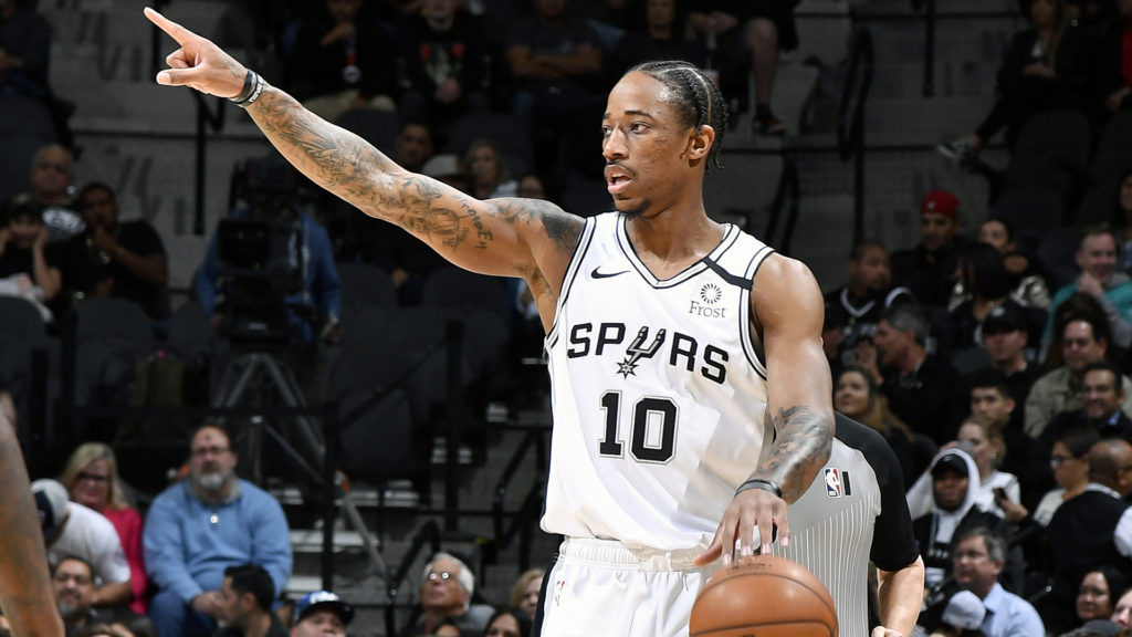
Last offseason, the Chicago Bulls traded for DeMar DeRozan, but which DeRozan exactly they were getting was unclear, as the former Toronto Raptors star was arguably declining and failed to make an all-star appearance in his three years in San Antonio. With that said, no one expected him to make the jump into the MVP discussion this season, let alone the Bulls’ early season success. How do you expect the unexpected anyways?

The consideration of expectation brings us into the sub-field of player projections and time-series forecasting. If we can analyze historical data in order to predict player performance from year to year, we can evaluate which players reached or failed to reach expectations, using statistical projections as a proxy. With this objective, I created a model to predict a player’s scoring output based on their statistics from the previous season.
Building the Model
Step 1: predictor variables
The first step in building the model is to determine which variables sufficiently influence how many points a player will score. I decided to select age, minutes, points, field goal percentage, three-point percentage, free-throw percentage, and usage rate as the predictor variables based off of intuition and preliminary exploratory data analysis (EDA). In other words, a young player who scores efficiently on high volume is more likely to improve his scoring output than an older player who shoots inefficiently on low volume.
Step 2: Training set


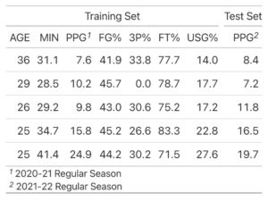
The next step is to find and clean data to train the model. I elected to scrape data from NBA.com over the past 20 seasons, filtering for players who appeared in at least half of the season (41+ games). Dropped from the training set as well are players without continuous data; if a player retired after the 2010 season, obviously there will be no improvement in 2011 so the 2010 data should be disregarded. Once all the data is retrieved, I standardized all values to prevent any one variable from being weighted more than the others since their original scales vary.
step 3: regression algorithm
The third and final step is to choose a regression algorithm for the model. I incorporated a random forest method, which consists of an ensemble of decision trees that contribute to an aggregated prediction for scoring output (here’s a great video explanation). Once the model is trained, we can use a test set to validate the model’s accuracy; I selected data from the 2020-21 season to “predict” scoring output for this past season. This model provides a quantitative means of comparing player expectations and actual performance, which takes us to the fun part: who outperformed expectations the most?
Model Results
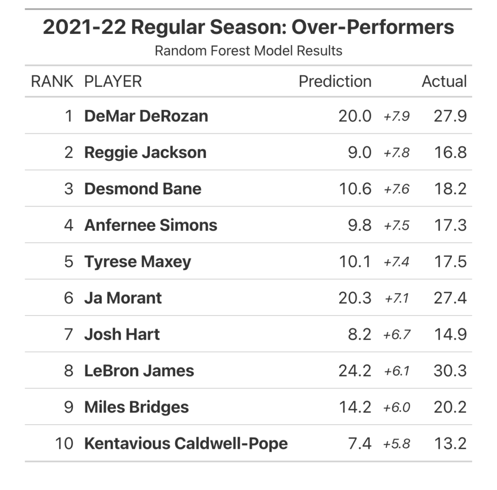
The table below highlights the top and bottom ten players who exceeded or failed to reach their scoring predictions. Unsurprisingly, veteran superstars DeRozan and James earned their respective ranks at first and eighth, with both of them actually projected to decrease in output, speaking to just how impressive their seasons were.


Outside of the top ten, a few notable players and their residuals – predicted points subtracted from actual points – are Dejounte Murray with 5.6 (11th), Jordan Poole with 4.8 (13th), and Tyler Herro with 3.8 (17th). The model goes both ways, and a few under-performers worth emphasizing are Stephen Curry with -2.9 (207th), De’Aaron Fox with -3.4 (217th), and Andre Drummond with -6.6 (249th). Note that the test set only includes 249 players.
Model Validation
When evaluating the accuracy of a regression model, two key metrics are used: R2 and root mean squared error (RMSE). R2 measures the proportion of variance that can be explained by the predictor variables on a scale from 0 to 1 – with 1 indicating a perfect fit – and RMSE is a measure of the variance – the standard deviation – of the residuals.

The R2 value was 0.79, which indicates a fairly strong correlation between the predictor variables and scoring output. The RMSE was 2.86, and the residual plot below shows a normal distribution around 0. The residuals are also independent of the response variable – points per game – which tells us that the model remains consistent regardless of how many points a player will score. In other words, an undesirable residual plot may show more variance when points exceed 30, which would imply that the model doesn’t predict high volume scorers’ output very accurately. This is not the case, and we can adequately trust the model and its results.
Conclusion
While validation metrics and basketball intuition back up the model, there are clear limitations and areas for growth. A more sophisticated model would incorporate more years of data in the training set, possibly from up to two or three years prior – this would place more weight on a player’s recent career trajectory into their projection. For example, a player who’s increased their scoring output for two years straight is more likely to continue on that upward path. Later iterations could also control for a player’s team composition or position, since the presence of multiple ball-dominant players could hinder any one player from making a sizable improvement. Similarly, a guard who simply has the ball in his hands more often than a rim-protecting big would likely have more potential to increase scoring output.

